
- First, the air is collected from the environment by the air source and brought to the compressor. At this point, the air acquires greater pressure, which also notably increases its temperature.
- Then, the air activates the outflow switch, choosing one direction or another depending on the irradiance.
- The next part of the process involves the fuel source and the combustor. In this part, the fluid acquires the temperature and the pressure needed to drive the turbine and the generator.
The objective of this project was to model and then optimize the physical processes that take place in this plant.
First, we needed to construct the data set. Here, we used Thermoflex, the leading developer of thermal engineering software, to collect historical data from all the variables into a single file. As always, the data was treated to fix faults and improve the quality.
Data set
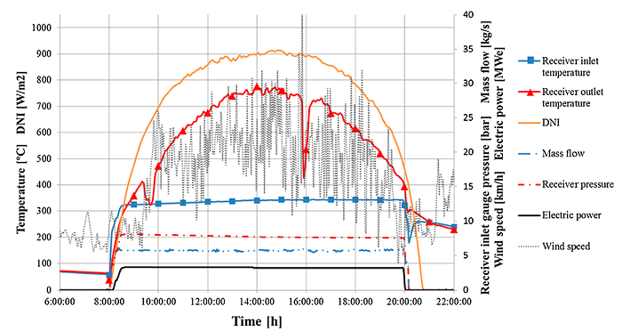
We compared real data obtained from the plant to the one our team calculated using Thermoflex. The following table shows the data obtained from the images, ambient variables for a nominal summer day, and the estimated fuel mass flow “Fuel Flow (T)” with its corresponding generated power values “P(T)”, so we can compare it to the real ones obtained from thermosolar “(S)”.
| Time (hour) |
Irradiance (W/m2) |
Temperature (K) |
Pressure (bar) |
R.H. (%) |
Air Flow (kg/s) |
Fuel flow (S) (Kg/s) |
Power (S) (MW) |
Fuel flow (T) (Kg/s) |
Power (T) (MW) |
|---|---|---|---|---|---|---|---|---|---|
| 7 | 0 | 289.079 | 1.0048 | 80 | 17.9 | 0.353 | 4.6 | 0.35 | 4.827 |
| 8 | 85 | 289.869 | 1.0043 | 80 | 17.9 | 0.346 | 4.6 | 0.34 | 4.813 |
| 9 | 240 | 291.579 | 1.0047 | 78 | 17.9 | 0.331 | 4.6 | 0.33 | 4.978 |
| … | … | … | … | … | … | … | … | … | … |
| 22 | 0 | 300 | 1.0046 | 80 | 17.9 | 0.346 | 4.6 | 0.35 | 4.729 |
- Ambient temperature: This variable describes the ambient temperature, making it a boundary variable. In this case, the unit is Kelvin (K). It has been set as an input variable.
- Relative humidity: This variable represents the percentage of humidity in the air, making it a boundary variable. This variable has been set as an input variable.
- Ambient pressure: It represents the ambient pressure at the moment, so it’s a boundary variable. Its unit is bar (bar) and it has been set as an input variable.
- Air flow mass: This variable represents the mass of air that passes per unit of time. It is a control variable and its unit is kg/s.
- Fuel flow mass: This variable represents the mass of fuel that passes per unit of time. It is a control variable and its unit is kg/s.
- Irradiance: The irradiance is the radiant flux (power) received by a surface per unit area. The SI unit of irradiance is the watt per square meter (W/m2). In this example, the irradiance is set as both an input and a boundary variable.
- Electrical power: This variable represents the output of the combined cycle power plant and is therefore a state variable. The unit is the megawatt (MW), and it is the target variable.
Modeling the physical process
The next step was to study the data and design the neural network. To do that, we applied different statistical methods. Studying the scatter charts, we could clearly see that the generated power increases linearly with the fuel flow mass. This is due to two things:
- On the one hand, as the total fluid flow increases, the power generated also increases.
- On the other hand, electricity generation is directly related to the temperature at which the fluid arrives at the turbine. Therefore, when more fuel is used in the plant, more heat is generated by the total fluid, and more power is generated by the plant.
Then, we studied the correlations between the variables and the target. The target depends on many inputs simultaneously, but it is interesting to look for linear dependencies among them. You can see the correlations in the following table:
| Generated power correlation | |
|---|---|
| Ambient temperature | 0.0091 |
| Relative humidity | 0.0426 |
| Ambient pressure | 0.0102 |
| Air mass flow | 0.152 |
| Fuel mass flow | 0.974 |
| Irradiance | 0.155 |
Neural networks
A surrogate model is an engineering method used when an outcome of interest cannot be easily measured directly, so a model of the outcome is used instead. Most engineering or physics problems require experiments or simulations to evaluate the objective and constraint functions in terms of control variables. In this case, the neural network represents our surrogate model.
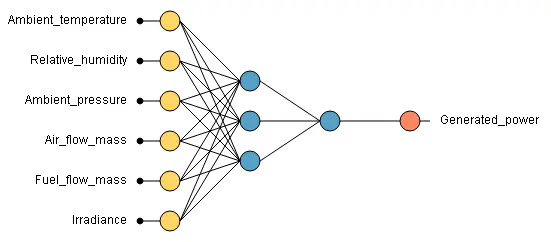
A graphical representation of the network architecture is depicted in the following picture. It contains a scaling layer, a neural network, and an unscaling layer. The yellow circles represent scaling neurons, the blue circles perceptron neurons, and the red circles unscaling neurons.
After building the neural network, it is necessary to train it to obtain the best possible performance. In this case, we applied the quasi-Newton training method.
We can see that the final selection loss and the final loss are very similar. If these two values were different, it would produce overfitting during the training.
Testing of the model
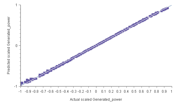
Once the predictive model has been trained, it is necessary to evaluate its predictive power on new data that it has not used before. This will assess the model’s quality and determine if it is good enough to move into the production phase; the grey line would indicate a perfect fit.
Another testing method that we can perform is error data statistics. With it, you can measure the minimums, maximums, means, and standard deviations of the errors between the neural network and the testing instances in the data set.
As shown in the previous table, the mean percentage error is 0.54751%, indicating that the model has good accuracy.
Once our predictive model is tested, we can use it to predict the generated power of the thermosolar plant whenever needed, based on the input variables.
Results
Optimal control is playing an increasingly important role in the design of modern systems. Its objective is the maximization of performance or the minimization of production costs.
Once we have modeled the physical system—in this case, the thermosolar plant production process—we can optimize it by minimizing fuel consumption, depending on other variables such as irradiance, ambient temperature, and ambient pressure.
After defining that our physical constraint will be generated power at 4.6MW, we have to determine the optimal (minimum) fuel flow to keep the generated power at the defined level by oscillating the airflow, which is a control variable.
In the following graph, you can observe the optimal fuel that the thermosolar plant should be using and the previous fuel that the plant was using.
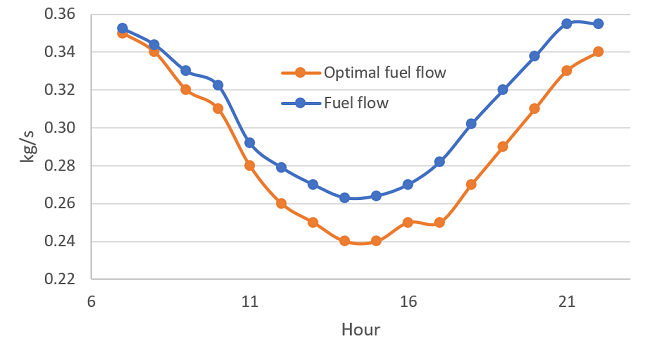
Using our artificial intelligence technology, the thermosolar plant managed to reduce fuel consumption, resulting in significant economic savings and improved plant performance.
| Concept | Amount |
|---|---|
| Daily fuel consumption (current) | 17779 kg/day |
| Daily fuel consumption (optimal) | 16668 kg/day |
| Yearly fuel savings | 405763 kg/year |
| Fuel price | 0.23 €/kg |
| Yearly money savings | 94870 €/year |